VictoriaMetrics Anomaly Detection: What's New in H1 2024?

With this blog post, we are excited to introduce a quarterly “What’s New” series to inform a broader audience about the latest features and improvements made to VictoriaMetrics Anomaly Detection (or simply vmanomaly). This first post will cover both Q1 and Q2 of 2024.

Stay tuned for the next content on anomaly detection

Releases

During the first half of 2024, we have released versions v1.8.0 through v1.13.3, which introduced:

• A new mode to address isolated observability tasks (so-called presets, e.g., for node-exporter-generated metrics).
• New models, such as MAD and AutoTuned, to broaden use case coverage and simplify model usage for users with limited Machine Learning knowledge.
• Domain-specific arguments such as detection_direction and min_dev_from_expected, allowing for fine-tuning of anomaly detection models to reduce false positives and better align with specific business needs.
• A mode for anomaly detection models to be dumped to a host filesystem after fit stage (instead of in-memory). Resource-intensive setups (many models, many metrics, bigger fit_window arg) and/or 3rd-party models that store fit data (like ProphetModel or HoltWinters) will have RAM consumption greatly reduced at a cost of slightly slower infer
• Enhanced support for multi-model, multi-scheduler, and multi-query configurations, enabling more flexible and resource-efficient setups.

We also improved our documentation, including additions to the FAQ, QuickStart, and Presets pages.

Let’s explore what these changes mean for our users.

Table of Contents

• Simplified Observability with Presets
• New Models Available
• Simplified Model Tuning with AutoTuned
• Fine-Tuning Anomaly Detection with Domain Knowledge
• Better Resource Management
• Flexible Configs

Simplified Observability with Presets

To further enhance the usability of vmanomaly, we have introduced a new preset mode, available from v1.13.0. This mode allows for simpler configuration and anomaly detection on widely-recognized metrics, such as those generated by node_exporter, which are typically challenging to monitor using static threshold-based alerting rules.

This approach represents a paradigm shift from traditional static threshold-based alerting rules, which focus on raw metric values, to static rules based on anomaly_scores. Anomaly scores offer a consistent, default threshold that remains stable over time, adjusting for trends, seasonality, and data scale, thus reducing the engineering effort required for maintenance. These scores are produced by our machine learning models, which are regularly retrained on varying time frames to ensure alerts remain current and responsive to evolving data patterns.

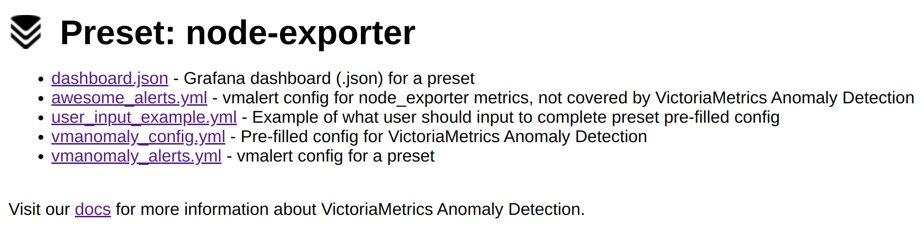
Additionally, preset mode minimizes the user input needed to run the service. You can configure vmanomaly by specifying only the preset name and data sources in the reader and writer sections of the configuration file. All other parameters are preconfigured. You also get additional assets, like Grafana Dashboard, Alerting rules and a Guide as a part of a preset:

Example configuration for enabling the node-exporter preset:

preset: "node-exporter"
reader:
  datasource_url: "http://victoriametrics:8428/" # your datasource URL
  # tenant_id: '0:0'  # specify for cluster version
writer:
  datasource_url: "http://victoriametrics:8428/" # your datasource URL
  # tenant_id: '0:0'  # specify for cluster version

Please refer to this page for more details about the presets and how to set up vmanomaly in node-exporter preset mode.

Return to ToC

New Models Available

We are continually enhancing vmanomaly to be more applicable to various anomaly detection use cases. In v1.8.0, we introduced the MAD (Median Absolute Deviation) model. This robust anomaly detection method is less sensitive to outliers compared to standard deviation-based models like ZScore. However, please note that models like MAD are best used on data with minimal seasonality and no trends.

Example model configuration using the MAD model:

# other config sections ...
models:
  your_desired_alias_for_a_model:
    class: "mad"  # or 'model.mad.MADModel' until v1.13.0
    threshold: 2.5
# ...

Return to ToC

Simplified Model Tuning with AutoTuned

We are committed to making vmanomaly as user-friendly as possible. Tuning the hyperparameters of a model can be complex and often requires extensive knowledge of Machine Learning. The AutoTunedModel is specifically designed to alleviate this burden. By simply specifying parameters such as anomaly_percentage within the (0, 0.5) range and tuned_class_name (e.g., model.zscore.ZscoreModel), you can optimize the model with settings that best suit your data.

Here are the key parameters to consider:

• tuned_class_name (string): The built-in model class to tune, such as model.zscore.ZscoreModel (or zscore starting from v1.13.0 with class alias support).
• optimization_params (dict): The only required argument is anomaly_percentage - an estimated percentage of anomalies that might be present in your data. For example, setting it to 0.01 indicates that up to 1% of your data points could be anomalous. More details and the intuition behind the AutoTuned mode can be found in the documentation.

Example model configuration using the AutoTuned model, wrapped around the built-in ZScore model:

# other config sections ...
models:
  your_desired_alias_for_a_model:
    class: 'auto'  # or 'model.auto.AutoTunedModel' until v1.13.0
    tuned_class_name: 'zscore'  # or 'model.zscore.ZscoreModel' until v1.13.0
    optimization_params:
      anomaly_percentage: 0.004  # required. Expecting <= 0.4% anomalies in training data
      seed: 42  # Ensures reproducibility & determinism
      n_splits: 4  # Number of folds for internal cross-validation
      n_trials: 128  # Number of configurations to sample during optimization
      timeout: 10  # Seconds spent on optimization per model during `fit` phase
      n_jobs: 1  # Parallel jobs. Increase if the fit window contains > 10,000 datapoints per series
  # ...

Return to ToC

Fine-Tuning Anomaly Detection with Domain Knowledge

To provide more precise and context-aware anomaly detection, vmanomaly has introduced domain-specific arguments such as detection_direction and min_dev_from_expected. These parameters help reduce false positives and align the model’s behavior with specific business needs.

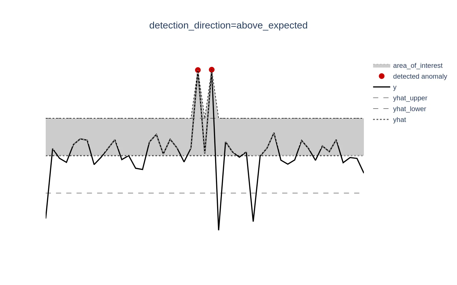
Introduced in v1.13.0, the detection_direction parameter allows users to specify the direction of anomalies relative to expected values. This is especially useful when domain knowledge indicates that anomalies are significant only when values deviate in a specific direction. The available options are: both, above_expected, and below_expected.

• Both: Tracks anomalies in both directions (default behavior). Useful when there’s no domain expertise to specify a particular direction.

• Below Expected: Tracks anomalies only when actual values (y) are lower than expected (yhat). Suitable for metrics where higher values are better, such as SLA compliance or conversion rates.

• Above Expected: Tracks anomalies only when actual values (y) are higher than expected (yhat). Ideal for metrics where lower values are better, such as error rates or response times.

Please find a graphical example below. y represents your actual data, yhat is a model prediction (expected value), [yhat_lower, yhat_upper] define a confidence interval around a prediction yhat. We can see data points values that are less that yhat_lower at the bottom part are not triggered as anomalies, because above_expected behavior was chosen.

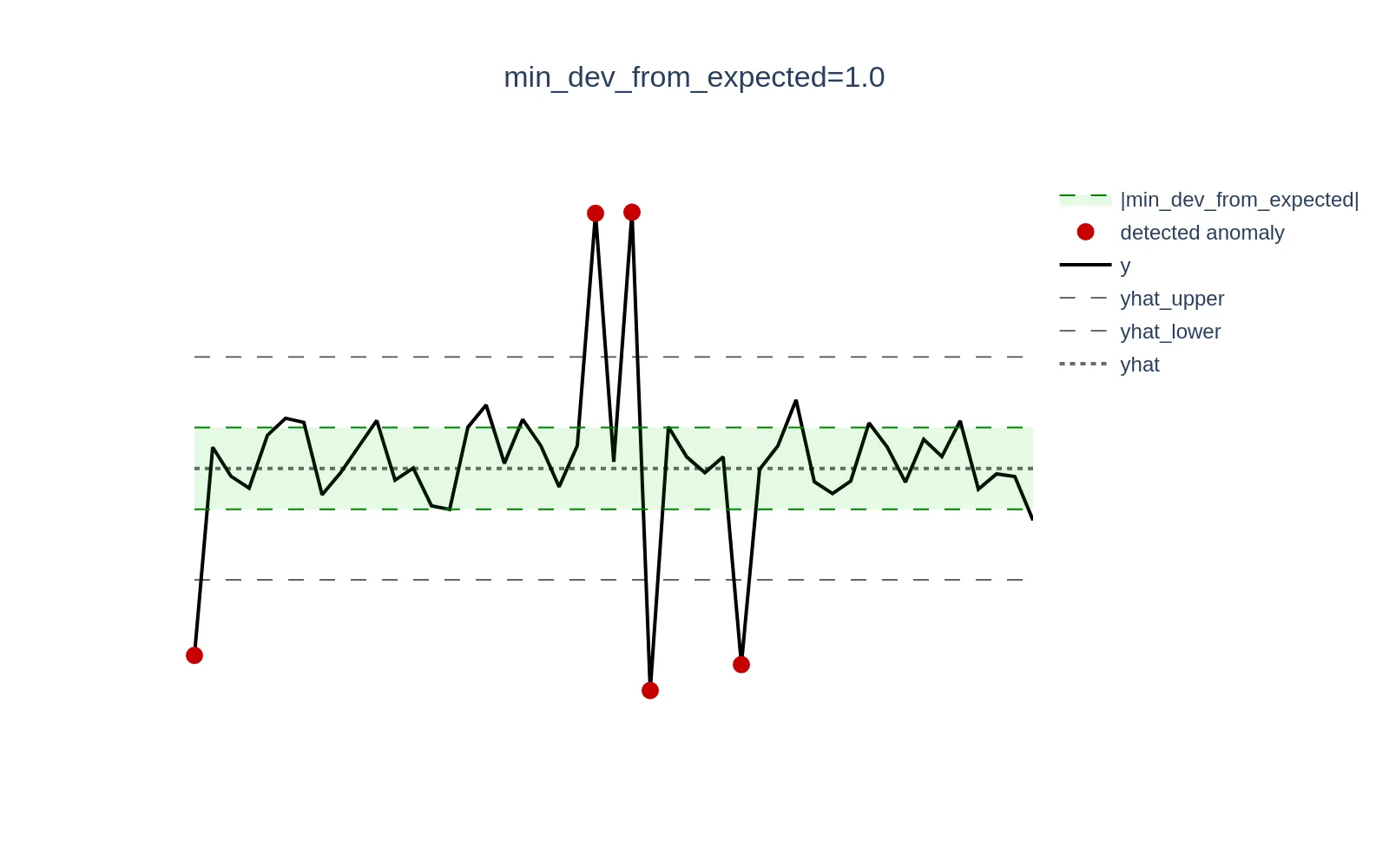
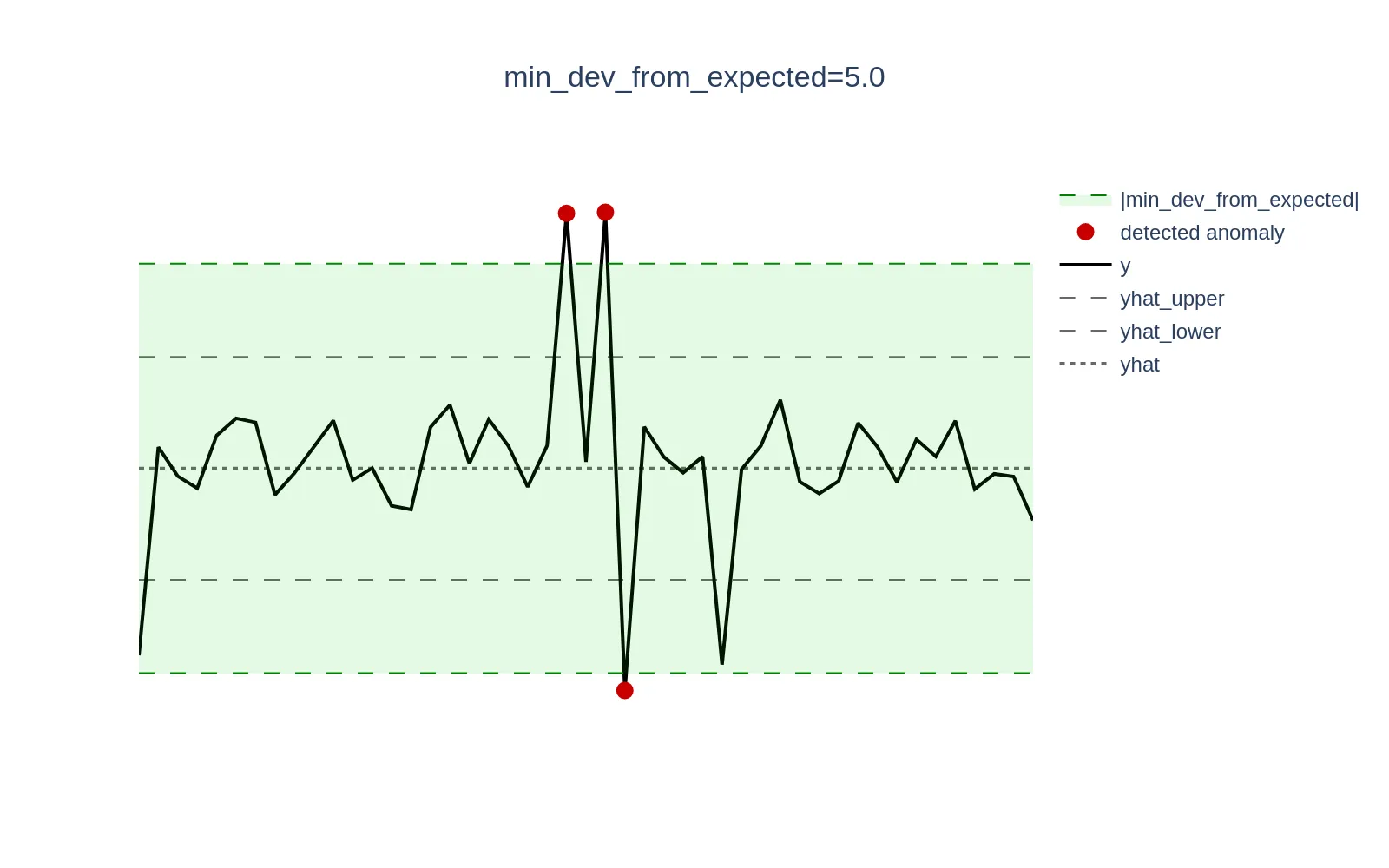
Also introduced in v1.13.0, the min_dev_from_expected argument helps in scenarios where deviations between the actual value (y) and the expected value (yhat) are only relatively high. Such deviations can cause models to generate high anomaly scores.

However, these deviations may not be significant enough in absolute values from a business perspective to be considered anomalies. This parameter ensures that anomaly scores for data points where |y - yhat| < min_dev_from_expected are explicitly set to 0 and won’t trigger any alerts that are based on anomaly scores.

The visualization below demonstrates this concept; the green zone defined as the [yhat - min_dev_from_expected, yhat + min_dev_from_expected] range excludes actual data points (y) from generating anomaly scores if they fall within that range. The higher the parameter, the wider green zone, the higher amount of data points will be excluded.

Let’s demonstrate how users can benefit from using such parameters on a simplified use case from one of our Engineers:

Currently I’m using the http_response and dns_query plugins in Telegraf to send data to VictoriaMetrics via the InfluxDB push protocol to monitor the health of the services in my homelab and meet the 99.9% uptime SLA in my wedding vows. It also makes my family/users less sad when they have issues since I’m usually working on an outage when the user reports it. Creating alerts and dashboards that track if something is up is simple but does not cover the service being slow. It is difficult to determine what slow means, especially across ~20 unrelated services, 4 dns servers, and no measurable definition of what slow is from the users. Determining this once is already a challenge, but as the environment changes from hardware upgrades, architecture changes, and services being added or removed this becomes nearly impossible.

To address the case, we ended up with such vmanomaly config:

schedulers:
  periodic:
    class: "periodic"
    infer_every: "1m"
    fit_every: "1h"
    fit_window: "6h"

models:
  mad:
    class: "mad"  # median absolute deviation
    z_threshold: 3.5
    detection_direction: 'above_expected'  # interested in peaks, not in dips
    min_dev_from_expected: 50.0  # not interested in anomalies |y - yhat| < 50ms 
    queries:
      - 'dns_blackbox'
      - 'http_blackbox'
    schedulers:
      - 'periodic'

reader:
  datasource_url: "http://victoriametrics:8428/"
  sampling_period: "1m"
  queries:  # in milliseconds
   dns_blackbox: 'avg by (server) (dns_query_query_time_ms[5m])'
   http_blackbox: 'avg by (server) (http_response_response_time[5m]) * 1000'
writer:
  datasource_url: "http://victoriametrics:8428/"

monitoring:
  pull:
    addr: "0.0.0.0"
    port: 8490

• The model chosen is MAD for being robust to outliers’ scale
• Users are interested only in increased latencies (vs expected behavior), thus, detection_direction arg is set to above_expected
• Users do not want alerts to be triggered if anomalies are small in absolute scale (vs expected values), that’s why we set min_dev_from_expected arg equal to 50 (ms). In production scenarios, it may be needed to set it higher, like 500ms or above.
• It has queries converted to the same scale (milliseconds), so min_dev_from_expected arg value is interpretable.

Here’s a couple of use cases, where anomaly score production was conditional:

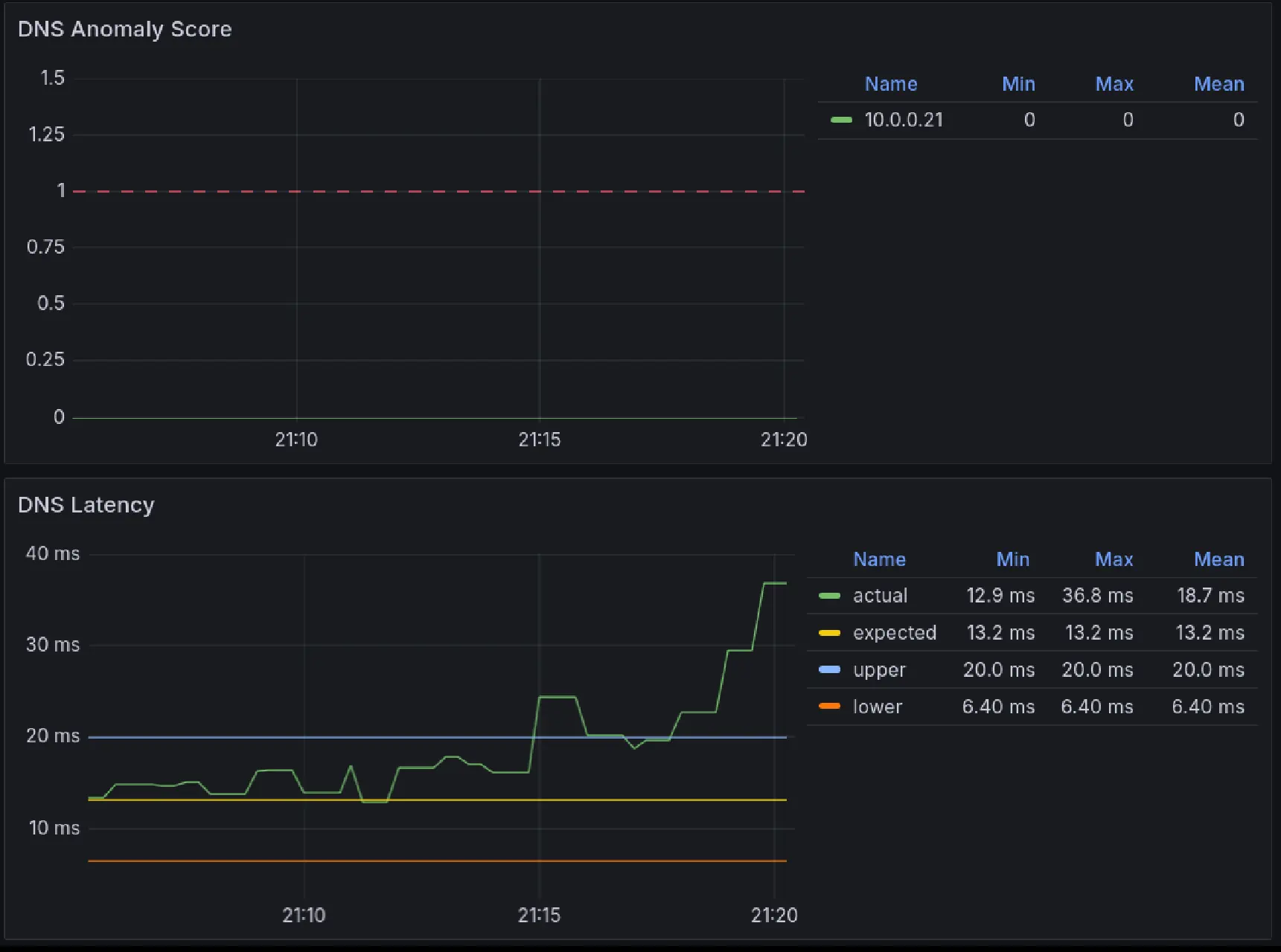
Case 1 (DNS Query Time)

We can see shift and pattern change around 21:15, but all anomaly scores remains 0 ( < 1), because

• metric value exceeds confidence boundaries: y > yhat_upper
• configuration has anomaly direction above_expected: y > yhat
• deviation didn’t exceed min_dev_from_expected: |y - yhat| <= 50ms

While it’s definitely an anomaly from technical perspective it’s not sufficient enough in absolute values to be considered a real anomaly (business perspective).

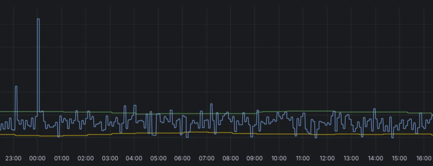
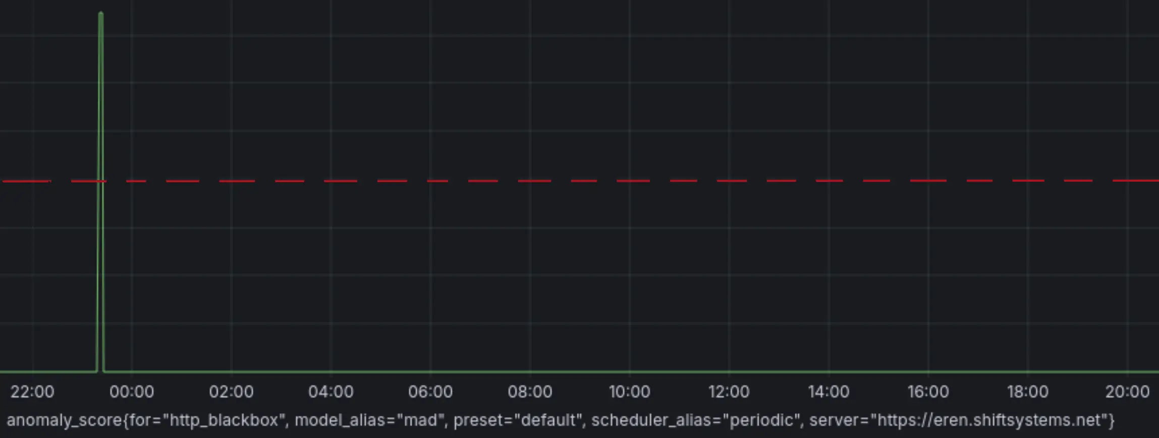
Case 2 (HTTP Response Time)

Anomaly around 00:00 was captured (anomaly score > 1), as

• (+) metric value exceeds confidence boundaries: y > yhat_upper
• (+) configuration has detection_direction=above_expected: y > yhat
• (+) deviation exceeded min_dev_from_expected: |y - yhat| > 50ms

Anomaly around 23:00 was not captured (anomaly score = 0), as

• (+) metric value exceeeds confidence boundaries: y > yhat_upper
• (+) has anomaly direction above_expected: y > yhat
• (-) deviation didn’t exceed min_dev_from_expected: |y - yhat| <= 50ms

Smaller anomalies were not captured for the same reason - the deviation didn’t exceeded min_dev_from_expected

P.s. the vmanomaly configuration and the blackbox health checks were deployed via shiftmon see their gitlab for more details.

Corresponding Grafana dashboard can be found here

Return to ToC

Better Resource Management

vmanomaly itself is a lightweight service, with resource usage primarily dependent on factors such as scheduling frequency, the number and size of timeseries returned by your queries, and the complexity of the employed models.

To deal with the latter, starting from v1.13.0, there is an option to save anomaly detection models on the host filesystem after the fit stage instead of keeping them in-memory by default. This is particularly beneficial for resource-intensive setups involving many models, numerous metrics, or larger fit_window values. Additionally, 3rd-party models that store fit data, such as ProphetModel or HoltWinters, will also benefit from this feature, significantly reducing RAM consumption at the cost of a slightly slower infer stage.

To enable on-disk model storage, set the environment variable VMANOMALY_MODEL_DUMPS_DIR to your desired location. The Helm charts have been updated accordingly to support this feature, with the use of StatefulSet for persistent storage starting from chart version 1.3.0.

Please find the example on how to set it up in Docker Compose using volumes here in FAQ

Return to ToC

Flexible Configs

Starting from v1.12.0, there exist many-to-many relationship between main config entities - queries (the data from VictoriaMetrics TSDB’s /query_range endpoint that vmanomaly operates on), models (that produce anomaly scores) and schedulers (that define how often the models should run its fit/infer stages). Together, it allows flexible configurations in a single vmanomaly service, to name a few use cases:

To define what queries to run a particular model on, see queries arg docs here. Different data subsets may expose different patterns, thus, requiring different model class to run on.

# other config sections ...
models:
  m1:  # model alias
    # other model params, like 'class'
    # i.e., if your `queries` in `reader` section has exactly q1, q2, q3 aliases
    queries: ['q1', 'q2']   # so `m1` model won't be run on results produced by `q3` query
    # if not set, `queries` arg is created and propagated 
    # with all query aliases found in `queries` arg of `reader` section
  m2:
    # other model params, like 'class'
    # i.e., if your `queries` in `reader` section has exactly q1, q2, q3 aliases
    queries: ['q3']   # so `m1` model won't be run on results produced by `q1`, `q2` queries

To split the models onto different schedulers. For example, simpler models might be retrained fit_every = each 1h on fit_window = 1d, while complex models may require bigger data frames and less frequent retrainings (i.e. fit_window = 1w and fit_every = each 1d). You can also attach the same models to multiple schedulers, if needed. See [schedulers] arg docs here.

# other config sections ...
schedulers:
  sc_daily:  # scheduler alias
    class: 'periodic'
    fit_every: '1h'
    fit_window: '1d'
    infer_every: '1m'
  sc_weekly:
    class: 'periodic'
    fit_every: '1d'
    fit_window: '7d'
    infer_every: '5m'
models:
  m1:  # model alias
    class: 'zscore'
    # if not set, `schedulers` arg is created and propagated 
    # with all scheduler aliases found in `schedulers` section
    schedulers: ['sc_daily']
    # other model args ...
  m2:  # model alias
    class: 'prophet'
    schedulers: ['sc_weekly']
    # other model args ...

To attach the same query to different models, i.e. to reduce false positives by composing smarter alerting rules with voting aggregation, like (avg(anomaly_score) by (for)) > 1, where for label, produced by writer holds a query alias, and the anomaly scores will be averaged for all the models that were attached to the query.

# other config sections ...
reader:
  class: 'vm'
  # other vmreader args ...
  queries:  # alias: MetricsQL expression
    q1: 'expr1'
    q2: 'expr2'
    q3: 'expr3'
models:
  m1:  # model alias
    class: 'zscore'
    queries: ['q1', 'q2', 'q3']  # list of aliases
    # other model args ...
  m2:  # model alias
    class: 'prophet'
    queries: ['q2', 'q3']  # list of aliases
    # other model args ...

Return to ToC

Would you like to test how VictoriaMetrics Anomaly Detection can enhance your monitoring? Request a trial here or contact us if you have any questions.