The Life of a Metric

Every number on your dashboards has a life story. It is born somewhere inside a running process, lives for a while as a few bytes in memory, travels across the network, settles down on a disk in some compressed shape, gets queried thousands of times, slowly loses its resolution as it ages, and is eventually deleted and forgotten forever.

If you have ever instrumented an application with metrics, the basic idea is familiar: you create a counter, you increment it, and somehow it shows up in a graph. This post fills in the “somehow” by following one single metric through that entire journey, using VictoriaMetrics as the storage backend. It is written for everyone (no programming background needed and no Go code to read), and if you want to go deeper, the VictoriaMetrics source is always the reference.

Let me introduce you to our metric.

One of the most common metrics out there is probably a counter of HTTP requests. Picture a single line in your service that runs on every request and bumps a number labeled with the request’s method, status, and path. Conceptually it is just:

http_requests_total{method="GET", status="200", path="/api/users"} 1027

This is a counter: a number that only ever goes up, until the process restarts and it resets to zero. http_requests_total is the metric name, the method, status, and path are labels, and 1027 is the current value. And here is the first thing you need to have crystal clear: every distinct combination of the metric name and the label values is a separate time series.

http_requests_total{method="GET", status="200", path="/api/users"} is one series. http_requests_total{method="POST", status="500", path="/api/users"} is a completely different one. That distinction follows our metric all the way down to the disk, so keep it in mind: a series is identified by its name plus the exact set of label values.

With the vocabulary settled, we can go back to the very start of the story: the moment a request comes in and our counter ticks up.

Here is the first thing that surprises people: when your code increments the counter, nothing leaves your process. No network call, no disk write, nothing. The metrics library just updates a number in memory.

Internally it keeps a small lookup table: for each set of labels it has seen, the running total for that label set. The first time it sees {method="GET", status="200", path="/api/users"}, it creates an entry with value 1. Every later increment of the same combination finds that entry and adds to it. For a counter, the library stores a cumulative total: the value keeps growing for the entire life of the process.

So at any given moment, your process is holding something like:

http_requests_total
  {method=GET,  status=200, path=/api/users}  -> 1027
  {method=POST, status=201, path=/api/users}  ->   84
  {method=GET,  status=500, path=/api/users}  ->    3

Three series, three integers, updated in place on every request. This is incredibly cheap, which is the whole point: you can instrument a hot path that runs millions of times per second and the overhead is essentially one table lookup and one addition.

But those numbers are useless if they never leave the process. So on a fixed interval, the values are exported: either the process is scraped (an agent fetches /metrics every 15–60 seconds) or it pushes a snapshot to a collector. Either way, the key mental model is the same:

Sooner or later, one of those periodic reports fires. Let’s follow it.

The moment the snapshot is taken, our series leaves home for the first time. It gets serialized (usually into Protocol Buffers) alongside its current value and the other metrics, and sent over HTTP to VictoriaMetrics. It can travel by any of several routes, because VictoriaMetrics understands several ingestion protocols natively, from Prometheus remote write to OpenTelemetry, InfluxDB, and Graphite, so whatever your stack emits, there is an endpoint waiting for it.

Besides the metric name and its labels, our data point carries just two more things that matter later: an absolute timestamp and the cumulative value at that moment. It does not announce “+500”; it announces “the total is now 1527, as of this instant.” That is exactly what VictoriaMetrics stores.

The trip is not always smooth. Maybe your storage server is down for some reason, or the network between you and it is misbehaving. To survive that, you can put an intermediary service in front of your storage that buffers messages until the road clears, for example vmagent. With it, our metric gets a safety net: vmagent buffers data in a disk-backed persistent queue, so even if the backend is unreachable, our data point waits patiently for hours and gets replayed once connectivity returns, instead of being lost on the road.

From here on, our metric has left your application. It is now VictoriaMetrics’ problem.

Whatever protocol the data arrived on, the first thing VictoriaMetrics does is translate it into one internal shape that the rest of the system understands: the request is decompressed, decoded, and flattened into simple (labels, timestamp, value) records. Part of that flattening is a small transformation that comes back to help us later: the metric name becomes a label. The name http_requests_total is stored as a special label called __name__, sitting right alongside method, status, and path. After this, a series really is just a set of labels.

By now, whether the data arrived via OpenTelemetry, Prometheus remote write, InfluxDB, or Graphite makes no difference anymore. Everything converges on the same representation:

{__name__="http_requests_total", method="GET", status="200", path="/api/users"}  ts=...  value=1527

And that tidy, human-friendly text form is exactly what VictoriaMetrics wants to get rid of first.

Text is easy for us to read, but expensive for a database to compare and store. So the labels get packed into a compact binary blob, the MetricNameRaw, roughly [len][name][len][value].... The packing is deliberately dumb: the labels go in in whatever order the client sent them, with no sorting, and the metric name itself is stored as just another label with an empty name.

For our series, the MetricNameRaw would look something like [0][19]http_requests_total[6]method[3]GET[6]status[3]200[4]path[10]/api/users (each length is really a 2-byte binary prefix, but you get the idea). Take the start, [0][19]http_requests_total: since the metric name is stored as the empty-named label, the [0] is that name (0 bytes long) and [19]http_requests_total is its value (19 bytes). Every other label follows the same [length][name][length][value] pattern. This blob is just a lookup key, though, not the real identity of the series; VictoriaMetrics builds that identity (from the labels in sorted order) later, only when it actually needs it.

That blob is still a fair amount of data to carry around for every single sample on disk and in every index. So here is the trick: instead of storing the whole thing, we pick a number (a 64-bit integer called the MetricID; under the hood, an always-growing counter seeded from the clock at startup, so it is unique within one storage instance), and with that plus a few other details we build a tiny fixed-size identifier, the TSID. From here on, inside storage the series is just that number: the TSID.

The catch, of course, is finding the right TSID for every sample that arrives, and finding it fast.

So now our metric arrives as a MetricNameRaw, and VictoriaMetrics has to answer a deceptively hard question: “is this a series I have seen before, or a brand-new one?” Turning a MetricNameRaw into a TSID is the single most frequent operation during ingestion, so it has to be as cheap as possible in the common case. VictoriaMetrics asks a series of increasingly expensive questions, and stops at the first one that answers. Here is the whole cascade at a glance:

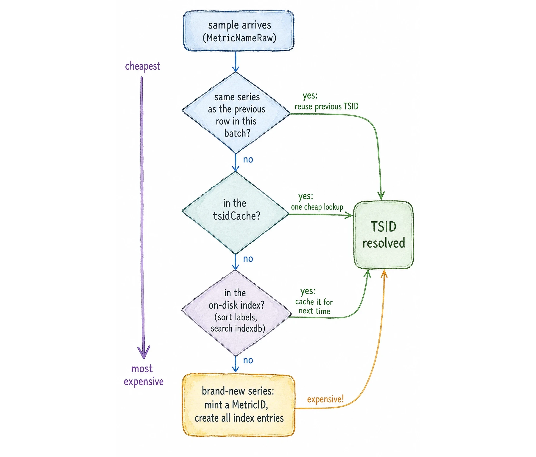
Let’s walk it top to bottom. The first question is the cheapest one: was the previous row in this batch the exact same series? If the MetricNameRaw is byte-identical to the row right before it, VictoriaMetrics simply reuses that TSID. In a normal scrape this rarely fires (each series usually shows up once per batch), but during bulk imports and backfills, where thousands of consecutive rows carry samples for the same series, it skips nearly all the work.

If the row before was different, the next question is: have we seen this series recently? VictoriaMetrics keeps an in-memory MetricNameRaw → TSID cache (the tsidCache). This is the single most important cache in the whole system, and on a warm instance our metric is almost certainly in there, so the answer usually costs a single cheap lookup.

If the cache does not have it, things get slower: do we have it written down anywhere? This is where the sorting finally happens: the labels are put into canonical order to build the canonical MetricName, and VictoriaMetrics goes to disk to search the on-disk inverted index for it.

And if even the index has never heard of it, then we have reached the last resort: this is a series nobody has ever seen before. This is the very first time this exact combination of labels exists. VictoriaMetrics mints a fresh MetricID for our metric and creates all the index entries for the new series.

The very first time your service emits http_requests_total{method="GET", status="200", path="/api/users"}, our metric falls all the way through to that final case. That step is dramatically more expensive than recording another sample of an existing series, and it is the root of every “high cardinality will hurt you” warning you have ever read. Let’s see why.

So our metric is brand-new, and being new is not free. Before anyone can query it, VictoriaMetrics has to make it findable, and that means writing it into the inverted index, which lives in its own store, the indexdb.

The easiest way to understand the index is to look at the questions it will have to answer later. Every kind of entry exists to answer exactly one of them:

The first three are cheap bookkeeping: one entry each. (The first row, by the way, is exactly the entry the “do we have it written down anywhere?” step of the previous section searches.) The real cost lives in the last two rows, the posting lists: for one specific label pair, the list of every series that carries it.

Being findable by any label means joining all the relevant lists. So our newborn metric gets added to the posting list for __name__="http_requests_total", and to the one for method="GET", and status="200", and path="/api/users" (four updates). Then three more for the composite name + label entries (http_requests_total with status="200", and so on), which exist because the most common query shape (a metric name filtered by a label) can then be answered from one single list. Seven updates for one new series.

And that is only half the bill. VictoriaMetrics also maintains per-day indexes: the same posting lists, but scoped to a single date. That is what makes “show me everything active in the last 3 hours” fast; a query over a narrow time window only has to look at the series that were actually alive on those days, not at everything that has ever existed. So each of those seven updates happens a second time, in today’s index: fourteen in total. Here is the full bill in one picture:

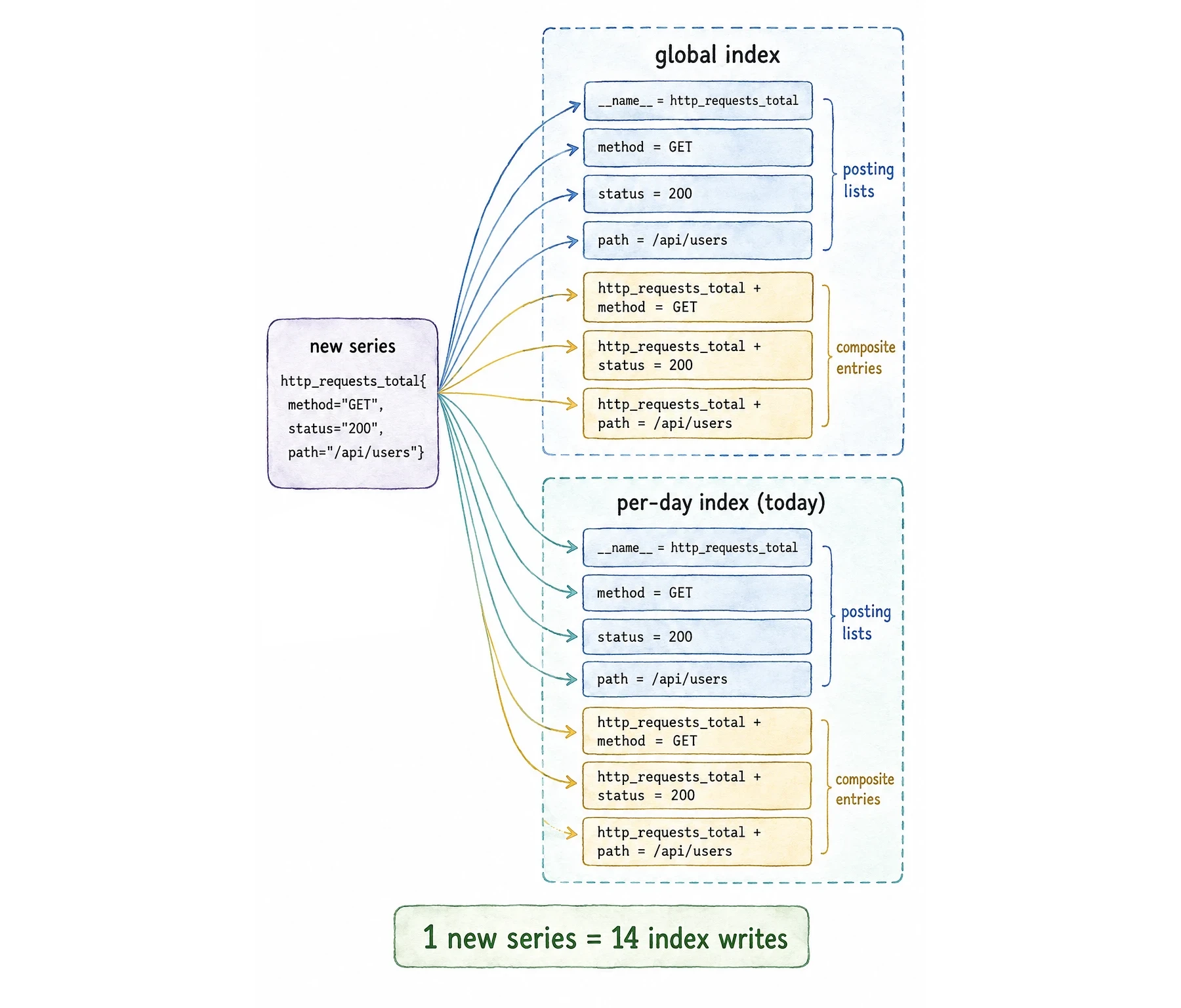
Fourteen writes for our newborn series; now compare that to its millionth sample later on, which costs almost nothing: it reuses a cached TSID and just appends a value. Being born is the expensive part of our metric’s life; growing up is cheap.

Once the index entries exist and the TSID is cached, our metric is officially “known”. But notice that everything so far has been about identity; we have not stored a single sample yet. Now its actual value needs to go somewhere.

VictoriaMetrics organizes data into monthly partitions, directories named YYYY_MM, and routes each sample to a partition by its timestamp. Within a partition, the write path follows a design known as an LSM tree (log-structured merge tree). The name sounds fancy, but the idea is simple: never modify existing data; always write new immutable files, and keep merging them into bigger ones in the background. It is a design tuned above all for one thing: ingesting an enormous number of samples per second.

The whole pipeline is built around one object: the part, VictoriaMetrics’ unit of physical storage (an immutable bundle of sorted, compressed samples). Every part has exactly the same internal format; the only things that change over its life are where it lives (RAM or disk) and how big it is. That is all the qualifiers mean: an in-memory part is a part still living in RAM, a small part is a freshly written one on disk, a big part is the result of merging many smaller ones.

With that in mind, here is the journey of our sample’s value once the series is known:

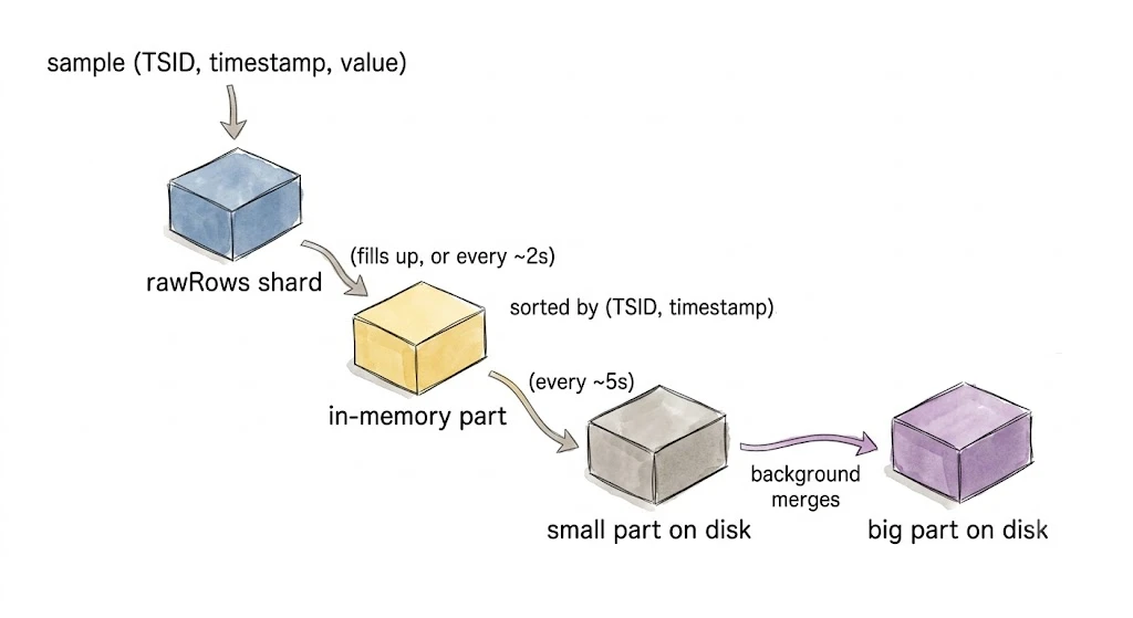
Our sample’s first stop is a rawRows shard: a plain in-memory buffer of a few megabytes, enough for a couple hundred thousand rows. There is one shard per CPU core, so ingestion threads never fight over a lock (a big deal when you are swallowing millions of samples per second).

It does not stay there long. When the shard fills up, or after a couple of seconds at most, everything in it gets sorted by (TSID, timestamp) and grouped into blocks: consecutive samples of the same series, up to 8192 of them, sitting physically next to each other. The blocks are then compressed into our sample’s first part, one still living in RAM: an in-memory part. This is the moment our sample stops being a loose row and takes on the columnar, compressed shape we will dig into next. It is also the moment it becomes visible to queries.

A few seconds later, a background flusher writes that in-memory part to disk as a small part, forcing the operating system to physically write the files rather than just promise to. This is the moment our metric becomes truly durable.

From then on, our sample rides the merge treadmill: dedicated workers continuously fold parts into bigger ones (in-memory parts into small parts, small parts into big parts, big parts into even bigger ones), always keeping everything sorted by (TSID, timestamp). Each merge also re-compresses the data more effectively: samples of a series that were split across several parts get consolidated into fuller blocks (up to a cap of 8192 samples each), and fuller blocks compress better than many partial ones.

So let’s recap what just happened to our metric. Its newest sample first landed in a buffer, mixed in with samples from thousands of other series, in whatever order they arrived. Moments later that buffer was sorted, and our sample ended up sitting right next to the other recent samples of its own series, as one block inside a part. A few seconds after that, the whole part was written safely to disk. And from now on, every time a merge runs, our sample’s block meets blocks of the same series coming from other parts, and they get folded together. Over the following hours, our metric’s samples keep gathering into fewer, bigger, better-compressed groups (which, as we will see, is exactly what makes reading them back fast). But before reading anything back, let’s look at what those compressed groups actually look like on disk.

Why does time series data compress so absurdly well? The answer starts with the layout. The heart of a part is just two files:

timestamps.bin   all the timestamps, compressed
values.bin       all the values, compressed

Two companion files, index.bin and metaindex.bin, act as the table of contents: they record which slice of those two files belongs to which series and time range, so a query can jump straight to the right bytes. (A small metadata.json rounds out the directory.) But the interesting story is in the two big files.

Notice that timestamps and values are stored separately. This is columnar storage, and it is the foundation everything else builds on. Instead of storing records like (ts1, v1), (ts2, v2), ... interleaved, you store all the timestamps together and all the values together. Why does that help? Because the numbers within a column are far more similar to each other than a timestamp is to its value, and similarity is exactly what compression feeds on.

Let’s take the two columns one at a time, timestamps first.

Metrics are usually sampled on a regular schedule: every 15 seconds, every 60 seconds. So a column of timestamps looks like:

1700000000000, 1700000015000, 1700000030000, 1700000045000, ...

Each of those is a big thirteen-digit number, but look closer: every one is exactly 15000 milliseconds after the previous one. All the interesting information is in the difference between neighbors, so why store the full numbers at all? Store the delta between consecutive timestamps instead and the column becomes 15000, 15000, 15000, .... Take the delta of the deltas (delta-of-delta) and you get 0, 0, 0, .... A column of zeros compresses to almost nothing.

The encoder is even smart enough to recognize the common cases explicitly. If every delta is identical, a whole block of thousands of timestamps is stored as just the first timestamp and the step. That’s it.

So much for the timestamps. The values are less predictable, so they need a little more machinery.

Values get a two-part treatment. First, floating-point values are converted into integers using decimal scaling: a value like 1.27 becomes a mantissa 127 with an exponent -2. Working with integers instead of raw floats makes the subsequent delta encoding far more effective. (The -precisionBits flag lets you trade a little precision for a lot more compression.)

Then the integers are delta-encoded, and here the shape of the series matters:

• A counter like our http_requests_total mostly climbs steadily, so delta-of-delta turns its values into a sequence of small, similar numbers, just like the timestamps.
• A gauge (say, CPU temperature) wanders up and down, so plain delta compresses it best.

VictoriaMetrics picks the right strategy per block.

After the delta encoding there is one final squeeze. The encoded stream is now full of small, repetitive numbers, and that is exactly the kind of input general-purpose compressors love. So VictoriaMetrics runs it through zstd (Zstandard): a fast, general-purpose compression algorithm. If zstd does not manage to shrink a given block by at least about 10%, the plain delta-encoded bytes are kept instead. Every block records which encoding it used, so the reader knows how to reverse it.

At this point our metric is at rest: a few bytes inside a compressed block, inside a values.bin, inside a part, inside a monthly partition, on a disk. It is durable, it is tiny, and it is ready to be read.

All this engineering just to store a number, but storage is only half the story. The whole point is to ask questions like:

rate(http_requests_total{status="500"}[5m])

“How many 500 errors per second, over the last 5 minutes?” Let’s trace it.

Before doing any heavy lifting, VictoriaMetrics checks whether it has answered this question recently. Query results are cached, so if you ran the same query 30 seconds ago (which is exactly what a Grafana dashboard on auto-refresh does), most of the answer is already sitting there, and only the newest slice of the time range actually needs to be computed. A dashboard refreshing every 30 seconds is not recomputing six hours of history each time; it is topping up a cached result.

So the cache really decides how much raw data must be fetched: if it has nothing, the whole time range; if it has a partial answer, only the missing slice. Either way, for that missing piece the engine has to go get the raw data (walking the same path ingestion took, but backwards):

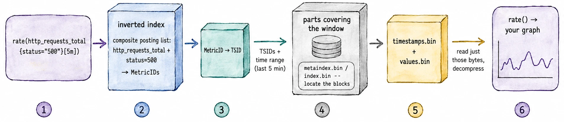
Let’s take it step by step. First, find the series. The query asks for http_requests_total{status="500"} (a metric name filtered by a label), which is exactly the shape the composite index entries were made for: a single posting list, written when our series was born, hands back every matching MetricID at once, and a quick hop through the MetricID → TSID entries turns those into TSIDs.

Then, get their samples. We now have a set of TSIDs and a time range: the last 5 minutes. With those in hand, VictoriaMetrics visits the parts covering that window, consults their table of contents (metaindex.bin and index.bin) to find exactly where the blocks of those series sit, and reads just those bytes from timestamps.bin and values.bin. The blocks are decompressed, undoing the encoding steps from the previous section, and the original timestamps and values come back out.

Finally, do the math. The rate function runs over the recovered samples, turning those ever-growing counter totals into the per-second rate you asked for.

This is exactly why we stored cumulative values all the way back at ingestion: the raw data stays simple (just the cumulative totals), and rates are derived on demand at query time. The result is rendered as JSON and sent back to Grafana, which draws your line. Our metric has now completed a full round trip: born in memory, persisted to disk, and read back out. It will repeat that loop thousands of times; meanwhile, quietly, it starts to age.

Our metric might be scraped every 15 seconds. That resolution is wonderful when you are debugging an incident today. But do you really need 15-second resolution for a metric from eight months ago? Almost never. At that age you care about trends (“was traffic higher last quarter?”), not individual 15-second blips.

Downsampling thins the data out as it ages, riding on the same background-merge machinery we already met. You might keep 15-second data for a week, then collapse it to 1-minute resolution for a month, then 15-minute resolution for a year. Each step throws away points but keeps the shape of the curve, so old data takes a fraction of the space while remaining correct for the questions you would actually ask of it.

There is no averaging or clever math involved. During merges, for each series, VictoriaMetrics keeps the last sample of each downsampling interval and simply discards the rest. For our counter this is remarkably safe: every sample is a cumulative total, so the last sample of a 15-minute interval already “contains” everything that happened during those 15 minutes. Dropping the samples before it loses the fine detail, but the totals (and therefore the rates you compute over old data) stay correct.

So as our metric ages, its once-dense stream of 15-second samples quietly thins out, merge after merge, until a whole day of history is just a handful of points. It is still our metric, still correct, just lower resolution. It is getting old.

Nothing lives forever, and you do not want it to; unbounded data means unbounded disk bills. VictoriaMetrics enforces a retention period (-retentionPeriod, one month by default) and removes data older than that.

This is where the monthly-partition layout pays off one last time. Because all the data for a given month lives in its own YYYY_MM directory, expiring old data is mostly a matter of deleting whole partition directories once every sample inside them is past the retention period. There is no expensive row-by-row scan to find what to delete; you just drop the month. As a finer backstop, merges also skip individual blocks whose newest timestamp has already fallen past the retention deadline, so expired data is not even carried forward into new parts.

And so, one retention period after its last sample, the partition holding our metric is deleted. The compressed bytes in values.bin are gone. The TSID, the inverted-index posting lists, the per-day entries, all eventually cleaned up. The series that started life as a single +1 in some request handler months ago is now, finally, gone. Lost forever, as if it never happened.

That is the full arc.

Let’s retrace the journey one last time, fast:

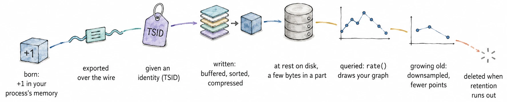
• Birth. Incrementing a counter just updates an integer in your process’s memory. Thousands of increments, no I/O. The value is exported only periodically.
• The wire. Each data point carries an absolute timestamp and the cumulative total, not a per-interval delta. vmagent’s disk-backed queue keeps your data safe during outages.
• Arrival. Every protocol is flattened to the same (labels, timestamp, value) shape; the name becomes the __name__ label and the series is just a set of labels from here on.
• Identity. Labels become a compact MetricNameRaw, which resolves (via a tiered cache) to a tiny TSID. A brand-new series triggers inverted-index writes for every label, the expensive part. Cardinality, not sample volume, is what costs you.
• Write path. Values flow through per-CPU buffers → compressed in-memory parts → durable parts on disk → ever-bigger parts via background LSM merges.
• On disk. Columnar storage splits timestamps from values; delta-of-delta and decimal+delta encoding plus zstd squeeze it to under a byte per sample.
• Query. A rate() query uses the inverted index to find the series, jumps straight to their blocks thanks to the sorted layout, decompresses them, and derives a per-second rate from the cumulative values.
• Old age and death. Background merges downsample aging data, and one retention period later the whole monthly partition is deleted.

The thing I find beautiful about this is how much of the cleverness is shared. The same LSM merge machinery that makes ingestion fast also does downsampling and retention enforcement. The same columnar layout that compresses the data also makes it fast to scan. The same TSID that saves space during writes makes the index small enough to keep in memory for reads. It is not a pile of separate features; it is a handful of good ideas, reused everywhere.

And it all started with a single +1.

This post stayed at altitude on purpose, so anyone could follow the whole arc without reading a line of Go. If you want to descend into the actual implementation, component by component, Phuong Le wrote an excellent series digging into the internals of each VictoriaMetrics component:

• How vmagent Collects and Ships Metrics Fast with Aggregation, Deduplication, and More and vmagent: Key Features Explained in Under 15 Minutes — the agent that collects and ships our metric.
• When Metrics Meet vminsert: A Data-Delivery Story — how the ingestion gateway parses, relabels, and routes data to storage.
• How vmstorage Handles Data Ingestion From vminsert and How vmstorage Processes Data: Retention, Merging, Deduplication,… — the write path, parts, and background merges up close.
• How vmstorage’s IndexDB Works — the inverted index and TSID resolution in detail.
• How vmstorage Handles Query Requests From vmselect and Inside vmselect: The Query Processing Engine of VictoriaMetrics — the read path, from selector to samples.