Prometheus Monitoring: Functions, Subqueries, Operators, and Modifiers

This discussion is part of the basic monitoring series, an effort to clarify monitoring concepts for both beginners and experienced users:

1. Counters, Gauges, Histograms & Summaries
2. Instant Queries and Range Queries Explained
3. Functions, Subqueries, Operators, and Modifiers (We’re here)
4. Alerting Rules, Recording Rules, and Alertmanager

We’re looking at 4 general types of functions here: rollup functions, aggregate functions, transformation functions, and label manipulation functions.

Rollup functions operate on a range vector. They take multiple data points over a time window and apply a function to reduce them to a single value. The result is an instant vector—one value per time series.

For example:

max_over_time(node_cpu_usage[3m])
step: 5m

This function looks at all data points collected over the past 3 minutes and returns the highest value to represent those samples.

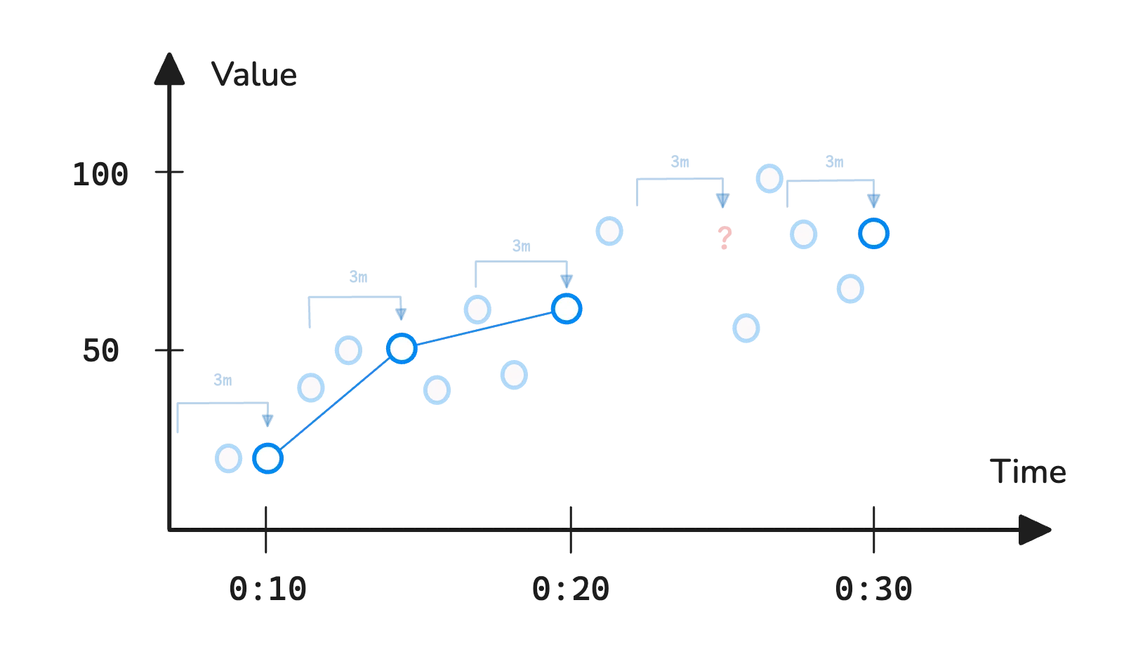
In the example above, max_over_time is evaluated at every 5-minute step between 00:10 and 00:30. Each time, it looks back over the previous 3 minutes, collects the samples, and returns the maximum value found in that range.

PromQL and MetricsQL both support many rollup functions. Here are some commonly used ones:

• rate(http_requests_total[5m]): Calculates the per-second average rate of increase over the last 5 minutes. Best used with counter metrics.
• increase(http_requests_total[5m]): Computes the total increase in the counter over the 5-minute window. Also used with counters.
• avg_over_time(http_requests_total[5m]): Returns the average value over the window. Works well with gauge metrics.
• sum_over_time(...), min_over_time(...), max_over_time(...): Similar to avg_over_time, but return the sum, minimum, or maximum values respectively.
• delta(temperature_celsius[5m]): Measures the difference between the first and last values in the range. Suitable for gauges.

You can explore more in the full documentation: https://docs.victoriametrics.com/metricsql/#rollup-functions

Remember: rollup functions require a range vector. If you forget the time window (for example, leave off [5m]) and pass an instant vector instead, PromQL will return an error. It’s basically saying, “I don’t know how much data you want me to roll up.”

MetricsQL handles this differently. If you forget the window and write:

rate(http_requests_total)

MetricsQL won’t throw an error. Instead, it tries to figure out the right window for you. It uses internal logic based on the query’s step, the scrape interval, and other context to choose a suitable time range automatically.

Aggregation functions are different from rollup functions. They don’t work across a time range. Instead, they combine multiple time series at a single point in time into one.

Imagine you have several services, and each tracks how many HTTP requests it handles using the http_requests_total metric. This metric includes labels like service and endpoint:

http_requests_total{service="auth", endpoint="/login"}       500 @ 00:10
http_requests_total{service="auth", endpoint="/logout"}      200 @ 00:10
http_requests_total{service="payments", endpoint="/checkout"} 350 @ 00:10
http_requests_total{service="payments", endpoint="/refund"}   150 @ 00:10
http_requests_total{service="inventory", endpoint="/items"}   400 @ 00:10
http_requests_total{service="inventory", endpoint="/stock"}   250 @ 00:10

If you’re not interested in the individual endpoint values, and just want to see the total number of requests each service handled, you can use:

sum(http_requests_total) by (service)

This groups the data by service and adds up the values. Other labels like endpoint are ignored. The output will look like:

http_requests_total{service="auth"}       700 @ 00:10
http_requests_total{service="payments"}   500 @ 00:10
http_requests_total{service="inventory"}  650 @ 00:10

Aggregation functions operate at a specific moment, not across a time range like rollup functions. Because of that, they require an instant vector (http_requests_total) as input.

And don’t forget what we covered in the previous article. When an instant vector like http_requests_total is evaluated, it gets internally converted to:

last_over_time(http_requests_total[lookback])

So, here’s how the full evaluation works:

1. The engine pulls all time series named http_requests_total within the given time range from the metrics storage
2. Converts the instant vector http_requests_total to last_over_time(http_requests_total[lookback]) (in Prometheus) or default_rollup(http_requests_total[lookback]) (in VictoriaMetrics)
3. Evaluates the last_over_time() or default_rollup() function at each timestamp to produce a full set of data points from 00:00:00 to 23:00:00
4. Applies the aggregation function sum() at each timestamp to group the values by service

So what happens if you run an aggregation query with a time window like this?

sum(http_requests_total[15m]) by (service)

Prometheus will return an error. That’s because aggregation functions expect an instant vector as input, not a range vector:

bad_data: invalid parameter "query": 1:5: parse error: expected type instant vector in aggregation expression, got range vector.

VictoriaMetrics handles this differently. It allows the query and gives you more control over the lookback window:

sum(last_over_time(http_requests_total[15m])) by (service)

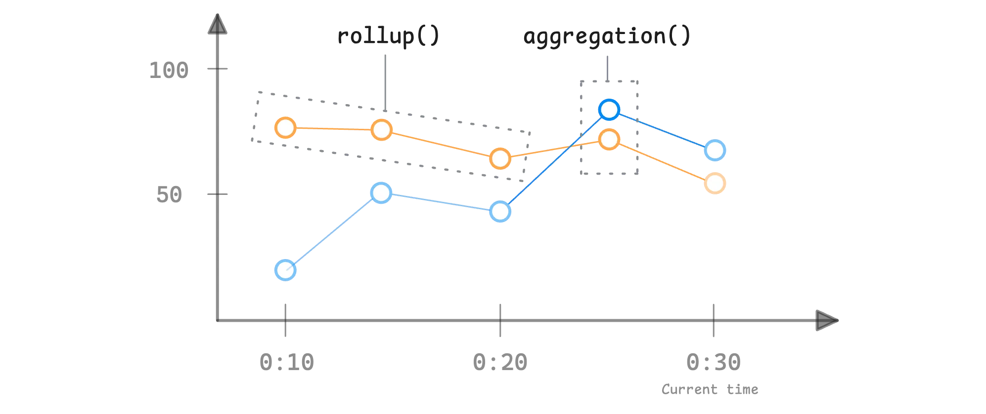
Now, to help you clearly understand the roles of aggregation and rollup functions, here’s a simple model:

aggregation_function(instant-vector) -> instant-vector
rollup_function(range-vector)        -> instant-vector

When using both together, it typically looks like this:

aggregation_function(rollup_function(range_vector)) -> instant-vector

Here’s a real-world example:

sum(rate(http_requests_total{job="api-server"}[5m]))
step: 1m

In this query, the system does the following:

1. Pulls all time series named http_requests_total in the given time range from the metrics storage.
2. Runs the rollup function rate(http_requests_total{job="api-server"}[5m]) to process the range vector and emit a data point.
3. Applies the aggregation function sum() to reduce it down by label.
4. Repeats step 2 and 3 every 1 minute to produce a full set of data points across the selected time range.

Note that step 2 and 3 happen for a single data point at a time, and this loop continues over the full time range. This is different from how a subquery works, which we will discuss very soon.

Now, here are some commonly used aggregation functions:

• avg: calculates the average across all time series
• count: returns the number of time series in the input
• max: finds the highest value at the current timestamp
• min: finds the lowest value across the series

For more, check out the docs MetricsQL - Aggregate Functions

Transformation functions are probably the easiest ones to get your head around. They don’t change the structure of the data—meaning, the number of time series and all the labels stay the same.

All they do is apply some kind of math to the sample values. Since they’re not working over time, they just take an instant vector as input and return an instant vector as output.

transformation_function(instant-vector) -> instant-vector

Here are a few common examples:

• abs(v instant-vector): takes the absolute value of each sample
• ceil(v instant-vector): rounds each sample up to the nearest whole number
• floor(v instant-vector): rounds each one down to the nearest whole number
• sqrt(v instant-vector): gives you the square root of each sample

Find the full list and details over at MetricsQL - Transformation Functions.

Label manipulation functions let you modify existing labels—or even create new ones—right inside your query. Two functions that tend to show up often are label_replace() and label_join().

They each work a bit differently:

• label_replace rewrites the value of dst_label using the value of src_label, but only if that source label matches a regex pattern.

  label_replace(v instant-vector, dst_label string, replacement string, src_label string, regex string)
  

• label_join combines the values of several labels using a separator, and stores that into a new label.

  label_join(v instant-vector, dst_label string, separator string, src_label_1, src_label_2, ...)
  

Let’s make this more concrete. Say we’ve got some data like this:

instance              http_requests_total
10.244.2.216:3000     165212

What we want here is just the IP part from the instance label, without the port. So we can use label_replace() to pull that out and store it in a new label called ip_address:

label_replace(
    http_requests_total, // input vector
    "ip_address",        // destination label
    "$1",                // replacement string
    "instance",          // source label
    "([0-9.]+):\\d+"     // regex pattern
)

The label_replace function uses the regular expression ([0-9.]+):\d+ to match an IP address followed by a port (like 10.244.2.216:3000), and captures just the IP part (10.244.2.216). The $1 replacement string inserts the first captured group (the IP) into the new ip_address label.

As a result, each metric with an instance label like 10.244.2.216:3000 will now also have an ip_address label set to just 10.244.2.216, while preserving the original metric value (http_requests_total = 165212):

instance              ip_address       http_requests_total
10.244.2.216:3000     10.244.2.216     165212

One thing to keep in mind, label_replace() doesn’t delete or rename the original label. It just adds a new one. If you actually want to overwrite the original, you can just set dst_label to be the same name as src_label, and the old value gets replaced.

Now, label_join() works the other way around. Instead of pulling from one label, it combines multiple labels into one:

label_join(
    http_requests_total, // input vector
    "endpoint",        // destination/new label
    "_",               // separator
    "method",          // source label 1
    "path"             // source label 2
)

Here, we’re creating a new label called endpoint, by sticking together the method and path labels with an underscore in between.

Before:

method   path    http_requests_total
GET      /bar    165212
GET      /foo    264472
POST     /bar    132268
POST     /foo    231344

After:

method   path    endpoint     http_requests_total
GET      /bar    GET_/bar     165212
GET      /foo    GET_/foo     264472
POST     /bar    POST_/bar    132268
POST     /foo    POST_/foo    231344

MetricsQL supports a variety of label manipulation functions, take a look at MetricsQL - Label Manipulation Functions for more details.

In earlier examples, we used a rollup function like rate() on a range vector, and then applied an aggregation function like sum() to combine multiple series. The structure looked like this:

sum(rate(http_requests_total[5m])) by (service)
step: 1m
start: 00:00:00
end: 23:00:00

This process generates one data point per minute for the entire range. Both rate() and sum() are applied at every step of the raw samples.

Subqueries invert the traditional order. Instead of writing the expression as aggregation(rollup(range-vector)), a subquery lets you do something like this:

// rollup(aggregation)
rate(sum(http_requests_total) by (service)[5m])
step: 1m
start: 00:00:00
end: 23:00:00

In this example:

• sum(http_requests_total) by (service) is the aggregation function. It sums up all matching series by service at each point in time.
• rate(...[5m]) is the rollup function. It calculates the per-second rate of increase over the last 5 minutes.

But there’s a catch: the sum(http_requests_total by (service)) expression returns an instant vector at each timestamp. For example, if you have two instances:

http_requests_total{service="server1"} 100 @ 00:00:00
http_requests_total{service="server2"} 200 @ 00:00:00

That’s just one snapshot in time. But rate(...) expects a range vector — multiple samples over time — not just one timestamp.

So how do we fix that?

Subqueries change how this evaluation works. They first run the inner expression (like sum(http_requests_total by (service))) over a full time range and generate a series of values. Only then does the outer rollup function like rate(...) process those results.

This way, the rollup function receives the full range of data it needs — not just a single moment — and can calculate properly.

Here is how this expression is evaluated step by step:

1. The system loads all http_requests_total time series samples within the selected time range.
2. The instant vector http_requests_total is automatically converted to last_over_time(http_requests_total[lookback]). (If you’re not sure how the lookback window is determined, see the previous article.)
3. At each 1-minute step, it evaluates both last_over_time(http_requests_total[lookback]) and sum(last_over_time(http_requests_total[lookback])) by (service) for the current timestamp.
4. After all sum() results are computed, the output is passed to rate() to calculate the per-second rate of increase over a 5-minute window.

At first glance, this seems fine. However, you might not realize that this rate(sum()) subquery construction is a common mistake. It can produce inaccurate results.

The issue is related to how counters behave. The rate() function is designed to work with counters, which increase over time but can reset to zero if a process restarts or crashes.

When rate() is applied directly to a raw counter, it can detect and handle resets correctly. But when you run sum(...) first, you lose that behavior. The aggregation hides individual resets from different series.

This means if one service restarts and another doesn’t, the reset will be hidden. As a result, applying rate() after sum() can produce inaccurate or misleading results.

To avoid this issue, it’s better to apply rate first, and then use sum, like the original query:

sum(rate(http_requests_total[5m])) by (service)

This keeps the counter behavior intact. Each time series is processed individually by rate() before being grouped by sum().

Now the next question is: how do you control the step of a subquery? For example, we want the inner query to run every 1 minute, and the outer query to run every 5 minutes.

To understand that, we need to look at how VictoriaMetrics handles step values in nested expressions:

• The inner rollup function inherits the step from the outer rollup function.
• The outer rollup function gets its step from the query input (usually from Grafana or vmui).

Take this example:

max_over_time(rate(http_requests_total[1m])[1m:30s])
step: 1m

In this case, even though the subquery defines a 30-second step inside the [1m:30s] window, it will be ignored. The actual step used will come from the outer step: 1m.

So here’s what happens:

Every 30 seconds, rate(http_requests_total[1m]) calculates the per-second rate of change for each time series using a 1-minute lookback window.

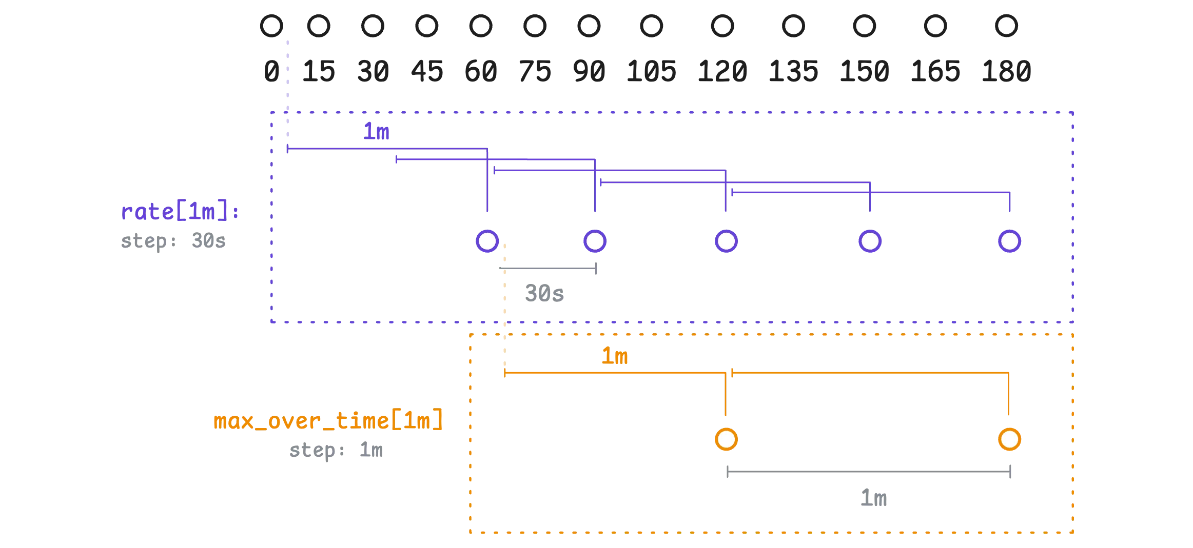
Then every 1 minute, max_over_time(...) collects those rate values and finds the maximum value within the last 1-minute window.

This pattern is helpful when you want to smooth out short spikes or highlight the highest values over a moving time window.

Up until now, we’ve mostly used the plain equality operator = when filtering time series—something like http_requests_total{method="GET"}. But the query language actually gives you a few more options for doing this kind of filtering.

• Inequality matcher (!=) filters out anything that matches the given value. For example, if you want to ignore any samples where the mode is "idle":

  node_cpu_usage{mode!="idle"}
  

• Regex matcher (=~) matches against a regular expression. So if you’re only interested in user and system modes:

  node_cpu_usage{mode=~"user|system"}
  

• Negative regex matcher (!~) excludes labels that match a regular expression. Let’s say you want to filter out both idle and iowait:

  node_cpu_usage{mode!~"idle|iowait"}
  

Just a note, if you filter with a condition like label="", it will match time series where the label exists with an empty value (label="") or where the label does not exist at all.

PromQL gives you a set of arithmetic operators: + for addition, - for subtraction, * for multiplication, / for division, % for modulo, and ^ for exponentiation. Same rules as regular math apply here—so things like multiplication and division happen before addition.

If you’re just using a scalar on one side of the operation, things are pretty straightforward:

http_requests_total / 10

Here, VictoriaMetrics applies that 10 to every value in every time series on the left. No matching needed, no overhead. It’s fast, efficient—each value just gets divided by 10 at every timestamp.

But when you’re working with two vectors—so, two sets of time series—it gets a bit more involved.

Now the system needs to figure out which time series on the left matches with which on the right. That’s where vector matching comes in.

Here is the setup:

cpu_usage{instance="server1", job="app"}
cpu_usage{instance="server2", job="app"}
cpu_limit{instance="server1", job="app"}

Let’s say we want to calculate CPU usage as a percentage of its limit:

cpu_usage / cpu_limit

Both metrics have the same label keys: instance and job. VictoriaMetrics looks at those and tries to match them up.

• For server1, both cpu_usage and cpu_limit exist with the same labels. So that series makes it into the result.
• For server2, we’ve only got cpu_usage—there’s no matching cpu_limit. So that one gets dropped.

In general, this pairing is done at each point in time—so the division happens only at timestamps where both series have data. If one side is missing a value at a certain timestamp, that point is skipped.

VictoriaMetrics also supports comparison operators: ==, !=, >, <, >=, and <=. These let you compare values between time series, one point in time at a time.

Just like with arithmetic operators, when you use these, the system tries to match time series from the left and right sides based on their labels.

Now, without any modifiers, VictoriaMetrics runs these comparisons in what’s called filtering mode:

• If the condition is true at a given timestamp, the value from the left-hand side is kept.
• If it’s false, the result becomes NaN—‘Not a Number’—and that point just disappears from the graph.

So if you run something like:

cpu_usage > cpu_requests

That’ll only show values where the left-side cpu_usage is greater than the right-side cpu_requests. Only the values that pass the comparison show up.

Here’s another one:

cpu_limit > 4

You’ll only see the actual values from cpu_limit when they’re above 4. Everything else is filtered out. But what if you don’t want to filter—what if you just want a yes-or-no signal?

That’s where the bool keyword comes in. It flips the behavior:

(http_requests_total >bool 100) 

Instead of keeping or dropping actual values, it returns a 1 if the comparison is true, and 0 if it’s not.

Finally, let’s consider operator precedence. The order in which things get evaluated. VictoriaMetrics gives priority to arithmetic operations first (*, /, +, -). Then it moves on to comparisons like == or >. And only after that does it apply logical set operations like and, or, or unless.

So with something like:

a + b > 10

It adds a and b first, then checks if the result is greater than 10.

Logical or set operators like and, or, and unless help you compare two sets of time series in a more structural way. Instead of doing math or comparisons on the values themselves, these work more like set operations: figuring out which series to keep, drop, or merge based on label matching.

This operator keeps only the time series that exist in both the left and right sides of the expression:

• If both sides have valid numbers at a given timestamp, the result keeps the value from the left side.
• If either side has a missing or invalid value (i.e., NaN), the result is NaN, and that point is dropped.

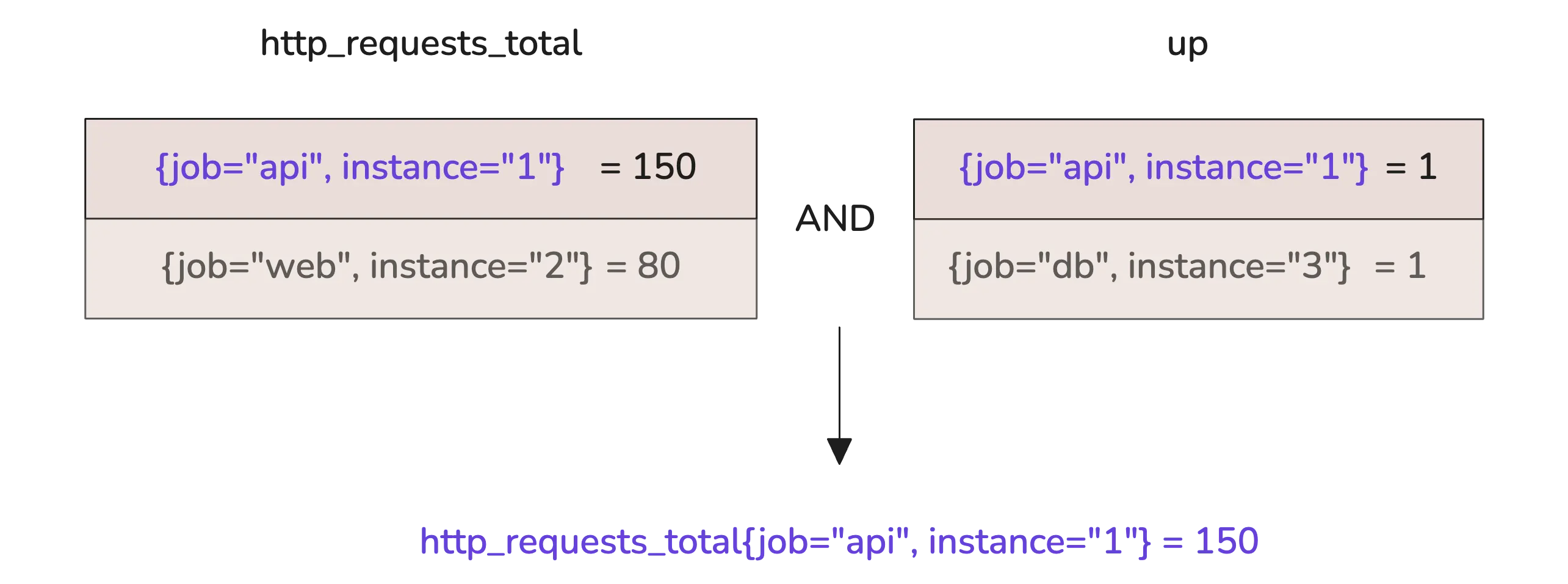
Say you run something like:

http_requests_total and up

If only {job="api", instance="1"} exists in both, that’s the only one that shows up in the result. Anything that doesn’t exist on both sides—like job="web" only being in http_requests_total, or job="db" only being in up—gets filtered out.

This one is more inclusive—it brings in time series from either side, as long as at least one of them has a valid value. If both sides match, the result takes the value from the left side.

So using the same setup:

http_requests_total or up

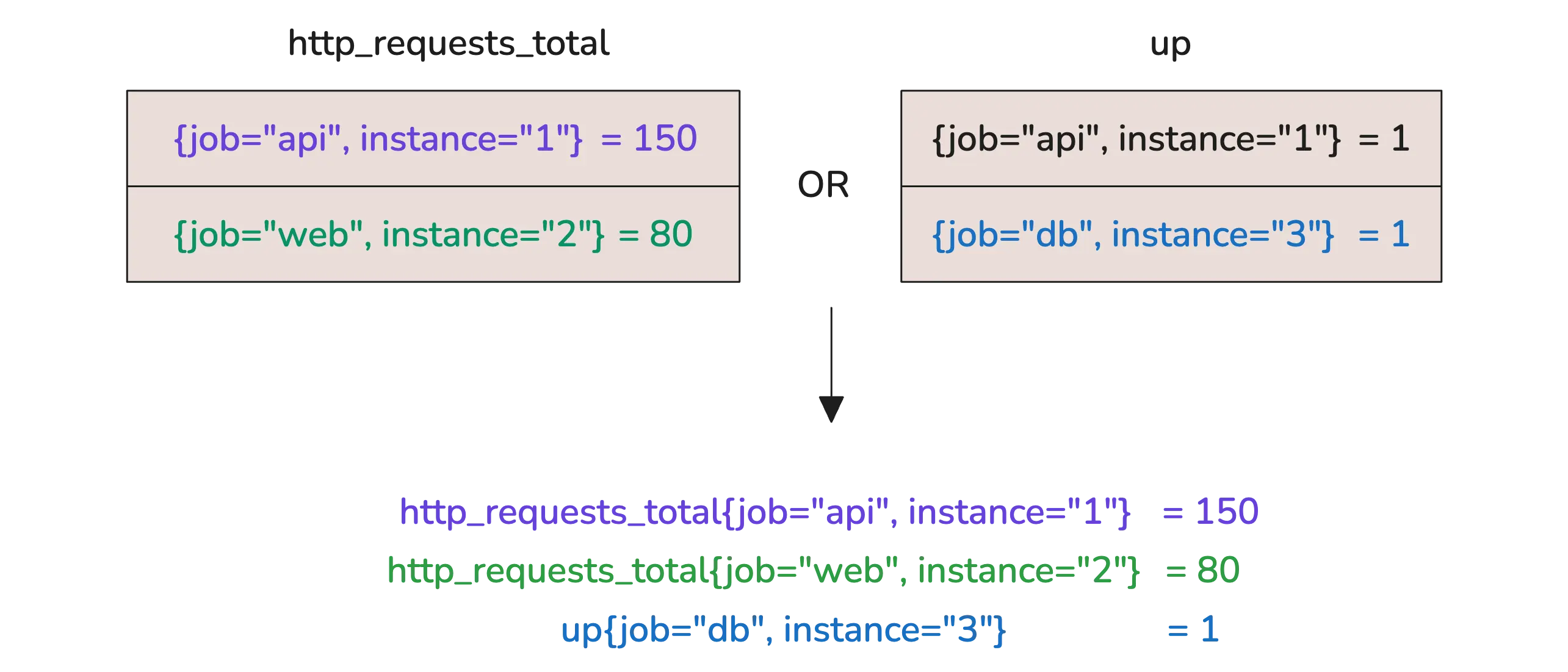
You’ll see all three jobs: api, web, and db. If a series only exists on one side, it’s still included. Think of it like a union—the widest possible set.

This flips the logic around. It keeps everything from the left side except the series that also exist on the right. So it’s like saying: “Give me all of these, unless they also show up over there.”

http_requests_total unless up

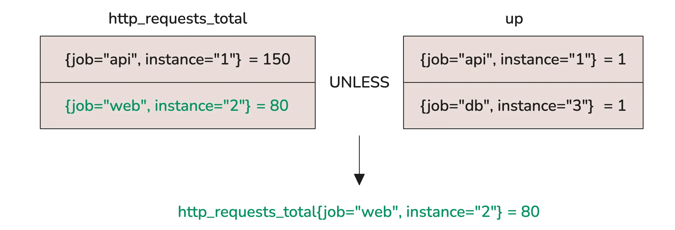
Here, the api series is dropped because it exists in both input vectors. What’s left is web, because it wasn’t matched on the right side.

In general, no matter which operator you’re using, the result always keeps the labels from the left-hand vector. So visually, everything still looks like it came from the left—even if the final set was shaped by what was on the right.

All the operators we’ve covered so far rely on label matching. That’s how the system figures out which time series from the left side should be paired with which on the right.

By default, it tries to match by all shared labels. That means even if just one label is different, that match won’t happen. That’s where the on(label_list) modifier becomes useful.

The on(...) modifier tells VictoriaMetrics to ignore all labels except the ones you list.

Only the selected labels will be used for matching. For instance:

metric_a{job="api", instance="1", region="us"}
metric_b{job="api", instance="2", region="eu"}

If you run a query like:

metric_a + metric_b

You’ll get nothing—no match, because the labels don’t line up. Now, if we say:

metric_a * on(job) metric_b

That works, because we’re telling VictoriaMetrics to only look at the job label when matching. But realistically, doing this with on(job) doesn’t give us much, because we could just use an aggregation function (avg, sum, etc.) like:

metric_a + avg by (job) (metric_b)

Same effect, less complexity.

The real value of on shows up in more involved cases, especially when we’re dealing with many-to-one or one-to-many matching.

All examples above have assumed one-to-one matching—each series on the left has exactly one match on the right. But what if two series on the left match a single series on the right?

This is many-to-one matching. And by default, it’s not allowed. To make it work, you’ll need to add group_left()—which tells VictoriaMetrics to keep all the left-hand series and match them to the single right-hand one:

http_requests_total * on(job) group_left() up

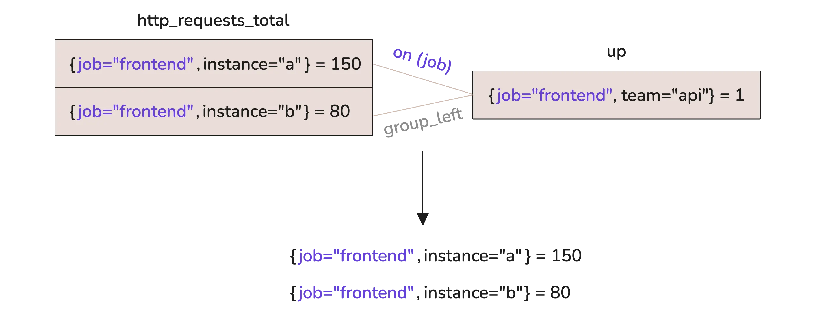
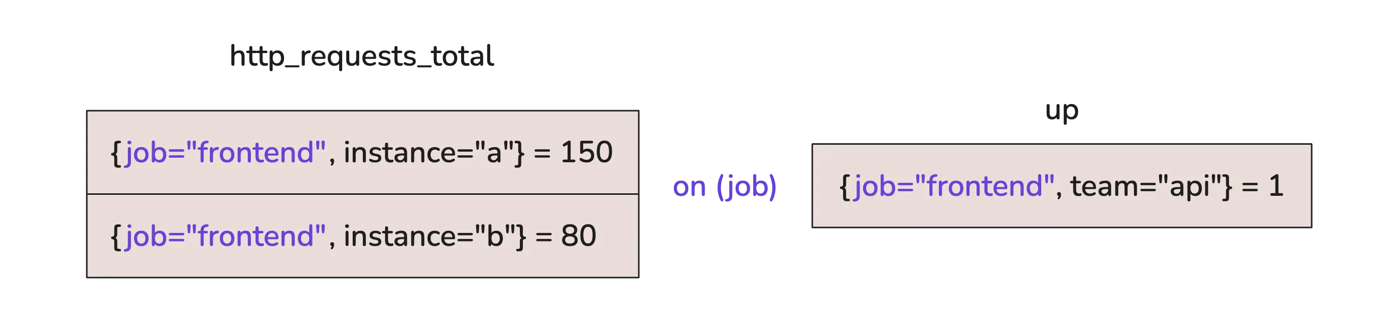
You’ll notice something, though. The team label from the right side is missing in the result. If you want to bring that over, you can add it inside group_left:

http_requests_total * on(job) group_left(team) up

That takes care of many-to-one. If you’re dealing with one-to-many, just flip it and use group_right().

Now, Prometheus doesn’t allow many-to-many matching—not even with group_left or group_right (except set operators and, or, unless). But VictoriaMetrics does, with one important condition: the final result must not have any duplicate time series. Every result must be uniquely identified by its label set.

Take this query:

http_requests_total * on(job) group_left() up

It leads to duplicate results because the label set isn’t unique:

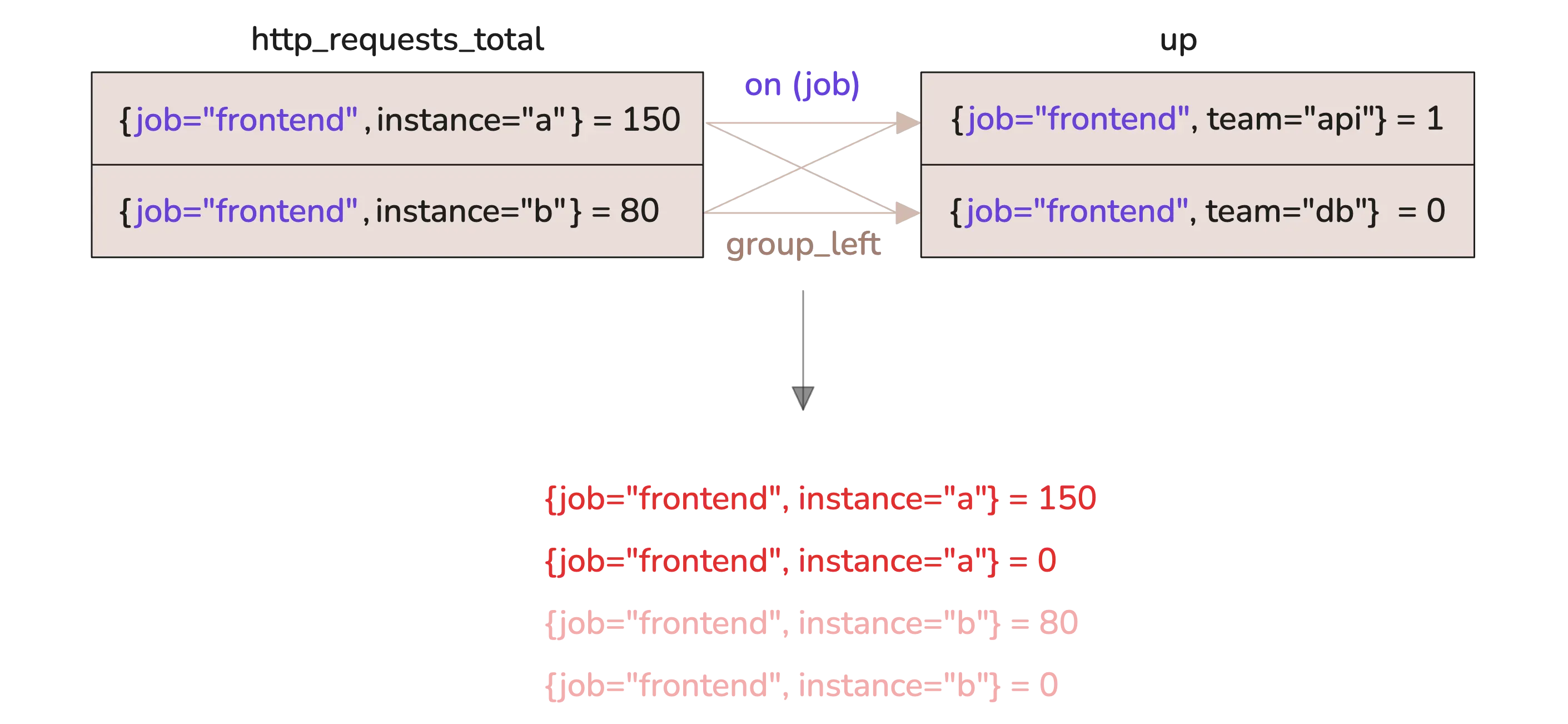
To fix that, just include a label from the right-hand side—something that makes each resulting series distinct:

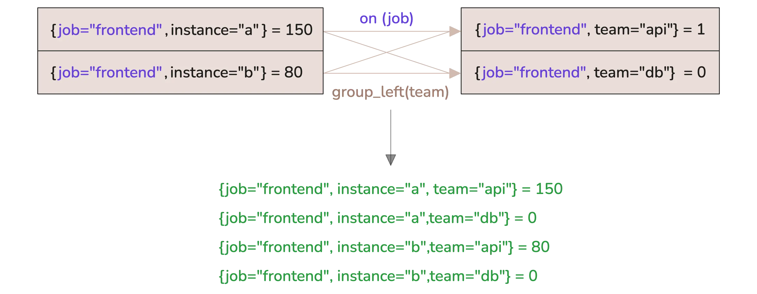
http_requests_total * on(job) group_left(team) up

Now the team label is preserved, and you still get 4 series in the result, but each one is uniquely labeled.

We provide a cost efficient, scalable monitoring and logging solution that most users are happy with. Check out VictoriaMetrics for more information.

If you spot anything that’s outdated or if you have questions, don’t hesitate to reach out. You can drop me a DM on X(@func25).